DAY 18 - Customer Sales Order Delivery Time Prediction Using Random Forest Regression - IT Consultant - SAP, Artificial Intelligence and Machine Learning

We have seen in our previous blog posts Customer Price Prediction on Machine Learning Scikit Learn Linear Regression and Random Forest models. To implement data intelligence, these models can be used in any SAP ERP, SAP ECC, SAP S/4 HANA, Oracle, Microsoft, or any ERP systems with a few custom function calls.

Also, we have gone through also Customer Sales Order delivery time/days prediction using the Machine Learning Scikit Decision Tree model and Scikit Linear Regression models.

In this post, we will work on Customer Sales Order Delivery time/Days Prediction using the Scikit Learn Linear Regression model (copied most of the codes from Customer Sales Order delivery time/days prediction) to check how it performs.

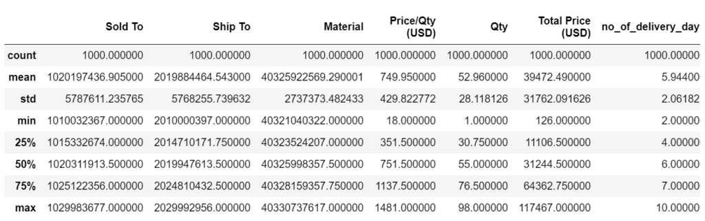
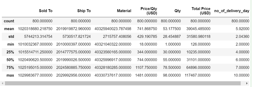
Let’s start and see how the Linear Regression predicts “Delivery days data” and you can also download from GitHub on my repository SODeliveryDaysPredictRandomForest.

Copy to Clipboard

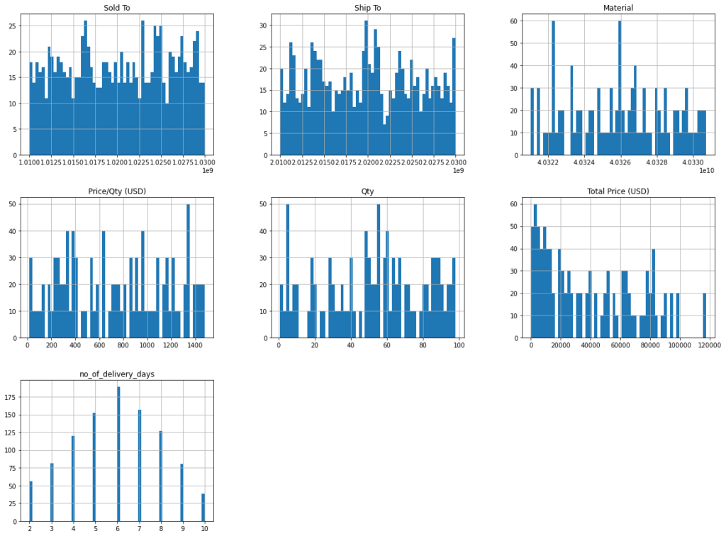
array([[<AxesSubplot:title={'center':'Sold To'}>,
        <AxesSubplot:title={'center':'Ship To'}>,
        <AxesSubplot:title={'center':'Material'}>],
       [<AxesSubplot:title={'center':'Price/Qty (USD)'}>,
        <AxesSubplot:title={'center':'Qty'}>,
        <AxesSubplot:title={'center':'Total Price (USD)'}>],
       [<AxesSubplot:title={'center':'no_of_delivery_days'}>,
        <AxesSubplot:>, <AxesSubplot:>]], dtype=object)

Copy to Clipboard

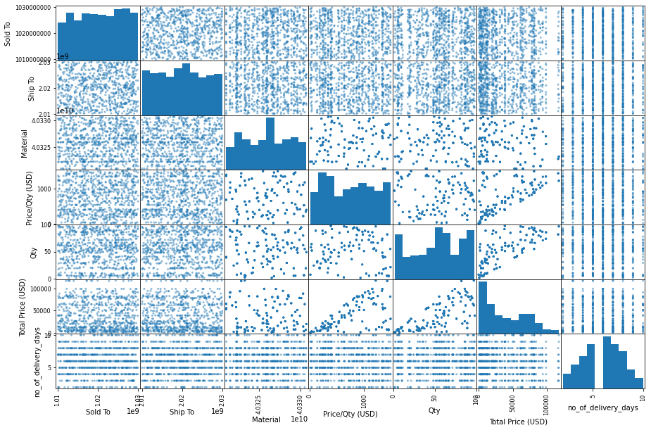
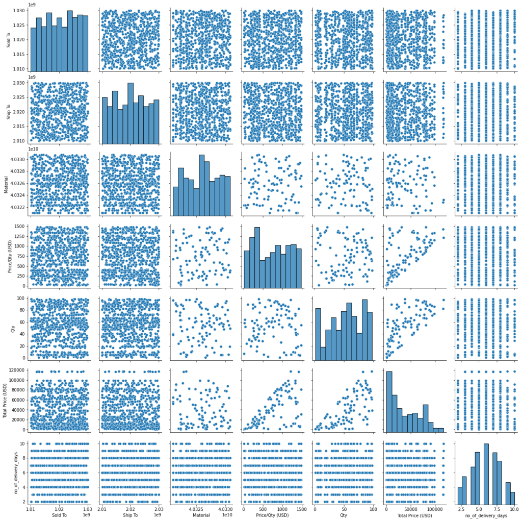
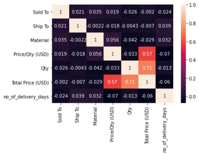
array([[<AxesSubplot:xlabel='Sold To', ylabel='Sold To'>,
        <AxesSubplot:xlabel='Ship To', ylabel='Sold To'>,
        <AxesSubplot:xlabel='Material', ylabel='Sold To'>,
        <AxesSubplot:xlabel='Price/Qty (USD)', ylabel='Sold To'>,
        <AxesSubplot:xlabel='Qty', ylabel='Sold To'>,
        <AxesSubplot:xlabel='Total Price (USD)', ylabel='Sold To'>,
        <AxesSubplot:xlabel='no_of_delivery_days', ylabel='Sold To'>],
       [<AxesSubplot:xlabel='Sold To', ylabel='Ship To'>,
        <AxesSubplot:xlabel='Ship To', ylabel='Ship To'>,
        <AxesSubplot:xlabel='Material', ylabel='Ship To'>,
        <AxesSubplot:xlabel='Price/Qty (USD)', ylabel='Ship To'>,
        <AxesSubplot:xlabel='Qty', ylabel='Ship To'>,
        <AxesSubplot:xlabel='Total Price (USD)', ylabel='Ship To'>,
        <AxesSubplot:xlabel='no_of_delivery_days', ylabel='Ship To'>],
       [<AxesSubplot:xlabel='Sold To', ylabel='Material'>,
        <AxesSubplot:xlabel='Ship To', ylabel='Material'>,
        <AxesSubplot:xlabel='Material', ylabel='Material'>,
        <AxesSubplot:xlabel='Price/Qty (USD)', ylabel='Material'>,
        <AxesSubplot:xlabel='Qty', ylabel='Material'>,
        <AxesSubplot:xlabel='Total Price (USD)', ylabel='Material'>,
        <AxesSubplot:xlabel='no_of_delivery_days', ylabel='Material'>],
       [<AxesSubplot:xlabel='Sold To', ylabel='Price/Qty (USD)'>,
        <AxesSubplot:xlabel='Ship To', ylabel='Price/Qty (USD)'>,
        <AxesSubplot:xlabel='Material', ylabel='Price/Qty (USD)'>,
        <AxesSubplot:xlabel='Price/Qty (USD)', ylabel='Price/Qty (USD)'>,
        <AxesSubplot:xlabel='Qty', ylabel='Price/Qty (USD)'>,
        <AxesSubplot:xlabel='Total Price (USD)', ylabel='Price/Qty (USD)'>,
        <AxesSubplot:xlabel='no_of_delivery_days', ylabel='Price/Qty (USD)'>],
       [<AxesSubplot:xlabel='Sold To', ylabel='Qty'>,
        <AxesSubplot:xlabel='Ship To', ylabel='Qty'>,
        <AxesSubplot:xlabel='Material', ylabel='Qty'>,
        <AxesSubplot:xlabel='Price/Qty (USD)', ylabel='Qty'>,
        <AxesSubplot:xlabel='Qty', ylabel='Qty'>,
        <AxesSubplot:xlabel='Total Price (USD)', ylabel='Qty'>,
        <AxesSubplot:xlabel='no_of_delivery_days', ylabel='Qty'>],
       [<AxesSubplot:xlabel='Sold To', ylabel='Total Price (USD)'>,
        <AxesSubplot:xlabel='Ship To', ylabel='Total Price (USD)'>,
        <AxesSubplot:xlabel='Material', ylabel='Total Price (USD)'>,
        <AxesSubplot:xlabel='Price/Qty (USD)', ylabel='Total Price (USD)'>,
        <AxesSubplot:xlabel='Qty', ylabel='Total Price (USD)'>,
        <AxesSubplot:xlabel='Total Price (USD)', ylabel='Total Price (USD)'>,
        <AxesSubplot:xlabel='no_of_delivery_days', ylabel='Total Price (USD)'>],
       [<AxesSubplot:xlabel='Sold To', ylabel='no_of_delivery_days'>,
        <AxesSubplot:xlabel='Ship To', ylabel='no_of_delivery_days'>,
        <AxesSubplot:xlabel='Material', ylabel='no_of_delivery_days'>,
        <AxesSubplot:xlabel='Price/Qty (USD)', ylabel='no_of_delivery_days'>,
        <AxesSubplot:xlabel='Qty', ylabel='no_of_delivery_days'>,
        <AxesSubplot:xlabel='Total Price (USD)', ylabel='no_of_delivery_days'>,
        <AxesSubplot:xlabel='no_of_delivery_days', ylabel='no_of_delivery_days'>]],
      dtype=object)

Copy to Clipboard

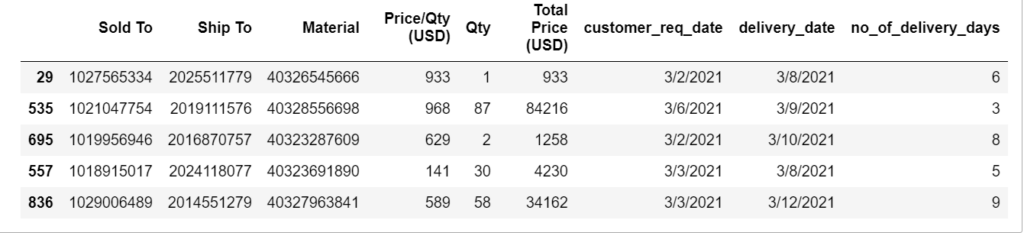
29     6
535    3
695    8
557    5
836    9
Name: no_of_delivery_days, dtype: int64

Copy to Clipboard

array([[ 1.26234643,  0.9764221 ,  0.22314994,  0.44560793, -1.83483918,
        -1.20757264],
       [ 0.12700257, -0.14113953,  0.96411821,  0.52720777,  1.18937949,
         1.43120235],
       [-0.06301307, -0.53241671, -0.97728689, -0.26314488, -1.79967385,
        -1.1972752 ],
       ...,
       [ 1.23018703,  1.18247717,  0.81514727,  1.37584601, -0.18206851,
         0.78864196],
       [-1.14424485, -1.45886269,  0.96411821,  0.52720777,  1.18937949,
         1.43120235],
       [-0.97055635, -0.566122  , -0.15123758, -0.48696156, -0.42822585,
        -0.54473421]])

Copy to Clipboard

array([[ 1.26234643,  0.9764221 ,  0.22314994,  0.44560793, -1.83483918,
        -1.20757264],
       [ 0.12700257, -0.14113953,  0.96411821,  0.52720777,  1.18937949,
         1.43120235],
       [-0.06301307, -0.53241671, -0.97728689, -0.26314488, -1.79967385,
        -1.1972752 ],
       ...,
       [ 1.23018703,  1.18247717,  0.81514727,  1.37584601, -0.18206851,
         0.78864196],
       [-1.14424485, -1.45886269,  0.96411821,  0.52720777,  1.18937949,
         1.43120235],
       [-0.97055635, -0.566122  , -0.15123758, -0.48696156, -0.42822585,
        -0.54473421]])

Copy to Clipboard

Random Forest Regression Delivery Time Prediction Y hat: [6.48 3.86 6.9  5.3  7.79 5.79 5.83 6.61 7.56 5.36]
Random Forest Regression Delivery Time Actual Y:  [6, 3, 8, 5, 9, 6, 6, 7, 8, 5]

Copy to Clipboard

Random Forest Delivery Time Mean Squared Error:  0.642017875
Random Forest Delivery Time Root Mean Squared Error:  0.8012601793425154

Copy to Clipboard

array([2.17277702, 2.04712115, 2.03528929, 2.19899011, 2.21883697,
       2.39311591, 2.13294954, 2.26850446, 2.27824494, 1.83581998])

Copy to Clipboard

Scores:  [2.17277702 2.04712115 2.03528929 2.19899011 2.21883697 2.39311591
 2.13294954 2.26850446 2.27824494 1.83581998]
Mean:  2.1581649377564682
Standard deviation:  0.14809743900088587

Conclusion on Scikit Learn – Linear Regression Model in Sales Order Delivery Time Prediction:

Random Forest Regression is a powerful model and compare to Linear Regression and Decison Tree, this is giving a best results as mean squared error 2.16 days.

Random Forest Regression model is performing well on delivery time prediction, however, we can compare pne more model with Neural Network and finalize the results.

The model is not overfitting the data very badly.

Random Forest Regression Scores shows in the range of 1.7 to 2.3 and Linear Regression Regression also same but Decision Tree shows 2.6 to 3.3.

We will check in Neural Network and come to final conclusion.

DAY 18 – Customer Sales Order Delivery Time Prediction Using Random Forest Regression