DAY 8 - Sales Order Delivery Days Prediction Using ML Decision Tree Regression - IT Consultant - SAP, Artificial Intelligence and Machine Learning

The decision trees are used to fit a sine curve with additional noisy observation. As a result, it learns local linear regressions approximating the sine curve.

We can see that if the maximum depth of the tree (controlled by the max_depth parameter) is set too high, the decision trees learn too fine details of the training data and learn from the noise, i.e. they overfit.

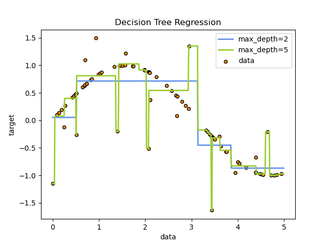
Reference and Image source: Scikit Learn

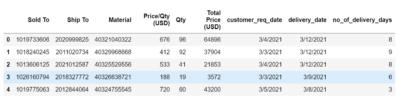
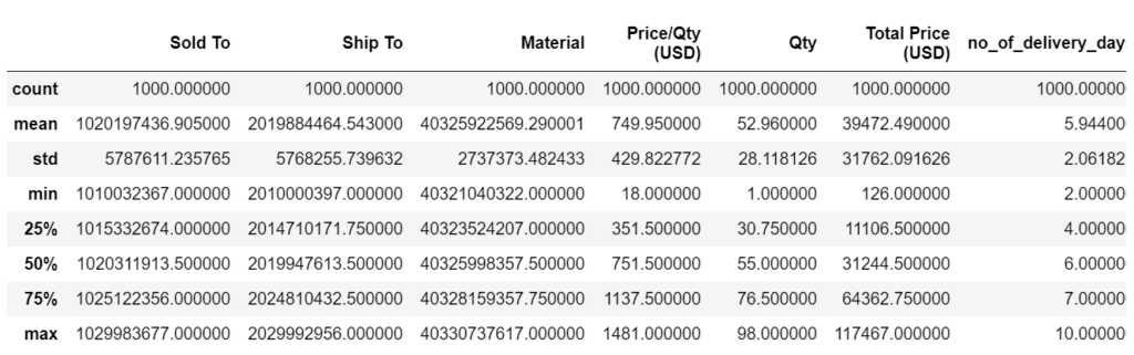
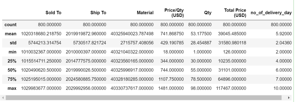
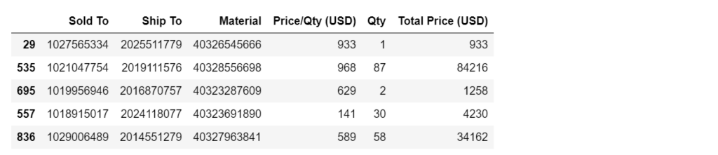
We can create a model Scikit Learn Decision Tree Regressor to check how it performs on Delivery Days Prediction. We have seen in our previous blog posts Customer Price Prediction on Machine Learning Scikit Learn Linear Regression and Random Forest models.

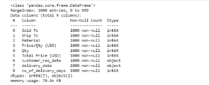
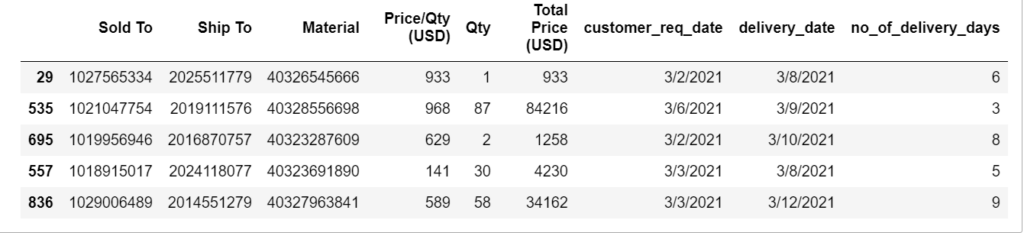
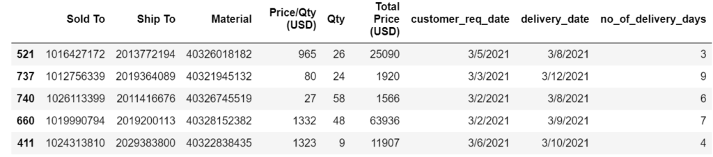
Let’s start and see how the decision tree predicts “Delivery days data” and you can also download from GitHub on my repository SODeliveryDaysPrediction

Copy to Clipboard

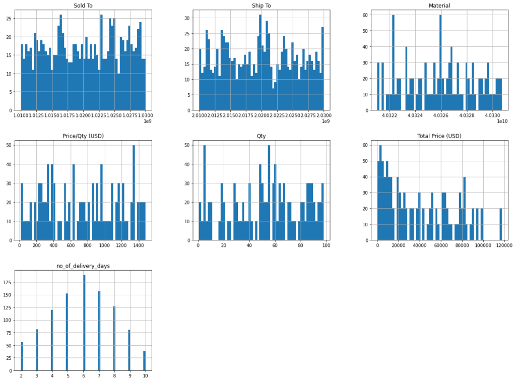
array([[<AxesSubplot:title={'center':'Sold To'}>,
        <AxesSubplot:title={'center':'Ship To'}>,
        <AxesSubplot:title={'center':'Material'}>],
       [<AxesSubplot:title={'center':'Price/Qty (USD)'}>,
        <AxesSubplot:title={'center':'Qty'}>,
        <AxesSubplot:title={'center':'Total Price (USD)'}>],
       [<AxesSubplot:title={'center':'no_of_delivery_days'}>,
        <AxesSubplot:>, <AxesSubplot:>]], dtype=object)

Copy to Clipboard

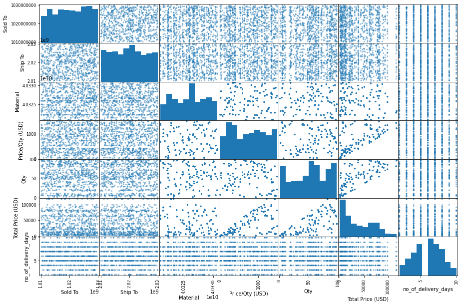
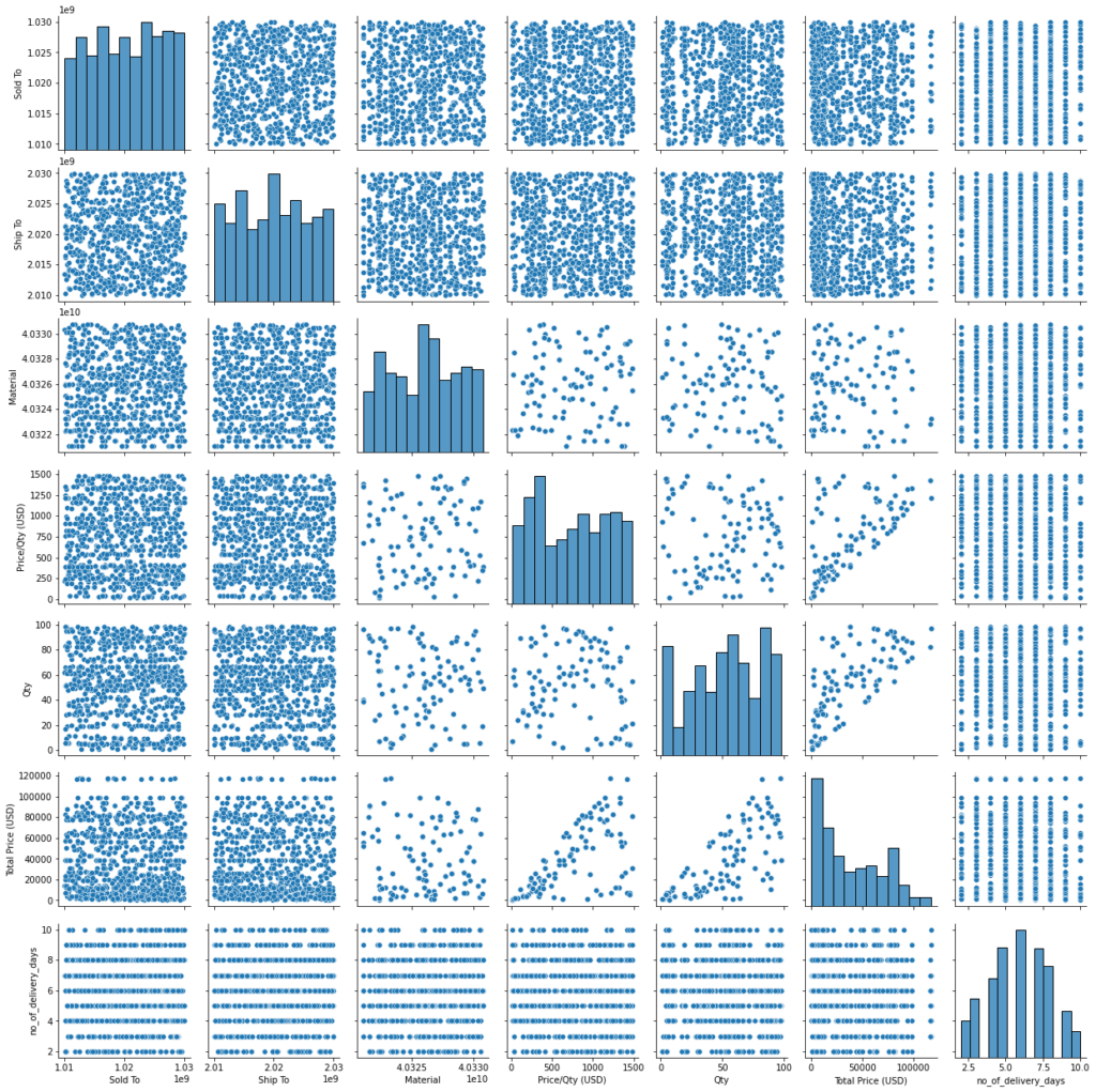
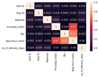
array([[<AxesSubplot:xlabel='Sold To', ylabel='Sold To'>,
        <AxesSubplot:xlabel='Ship To', ylabel='Sold To'>,
        <AxesSubplot:xlabel='Material', ylabel='Sold To'>,
        <AxesSubplot:xlabel='Price/Qty (USD)', ylabel='Sold To'>,
        <AxesSubplot:xlabel='Qty', ylabel='Sold To'>,
        <AxesSubplot:xlabel='Total Price (USD)', ylabel='Sold To'>,
        <AxesSubplot:xlabel='no_of_delivery_days', ylabel='Sold To'>],
       [<AxesSubplot:xlabel='Sold To', ylabel='Ship To'>,
        <AxesSubplot:xlabel='Ship To', ylabel='Ship To'>,
        <AxesSubplot:xlabel='Material', ylabel='Ship To'>,
        <AxesSubplot:xlabel='Price/Qty (USD)', ylabel='Ship To'>,
        <AxesSubplot:xlabel='Qty', ylabel='Ship To'>,
        <AxesSubplot:xlabel='Total Price (USD)', ylabel='Ship To'>,
        <AxesSubplot:xlabel='no_of_delivery_days', ylabel='Ship To'>],
       [<AxesSubplot:xlabel='Sold To', ylabel='Material'>,
        <AxesSubplot:xlabel='Ship To', ylabel='Material'>,
        <AxesSubplot:xlabel='Material', ylabel='Material'>,
        <AxesSubplot:xlabel='Price/Qty (USD)', ylabel='Material'>,
        <AxesSubplot:xlabel='Qty', ylabel='Material'>,
        <AxesSubplot:xlabel='Total Price (USD)', ylabel='Material'>,
        <AxesSubplot:xlabel='no_of_delivery_days', ylabel='Material'>],
       [<AxesSubplot:xlabel='Sold To', ylabel='Price/Qty (USD)'>,
        <AxesSubplot:xlabel='Ship To', ylabel='Price/Qty (USD)'>,
        <AxesSubplot:xlabel='Material', ylabel='Price/Qty (USD)'>,
        <AxesSubplot:xlabel='Price/Qty (USD)', ylabel='Price/Qty (USD)'>,
        <AxesSubplot:xlabel='Qty', ylabel='Price/Qty (USD)'>,
        <AxesSubplot:xlabel='Total Price (USD)', ylabel='Price/Qty (USD)'>,
        <AxesSubplot:xlabel='no_of_delivery_days', ylabel='Price/Qty (USD)'>],
       [<AxesSubplot:xlabel='Sold To', ylabel='Qty'>,
        <AxesSubplot:xlabel='Ship To', ylabel='Qty'>,
        <AxesSubplot:xlabel='Material', ylabel='Qty'>,
        <AxesSubplot:xlabel='Price/Qty (USD)', ylabel='Qty'>,
        <AxesSubplot:xlabel='Qty', ylabel='Qty'>,
        <AxesSubplot:xlabel='Total Price (USD)', ylabel='Qty'>,
        <AxesSubplot:xlabel='no_of_delivery_days', ylabel='Qty'>],
       [<AxesSubplot:xlabel='Sold To', ylabel='Total Price (USD)'>,
        <AxesSubplot:xlabel='Ship To', ylabel='Total Price (USD)'>,
        <AxesSubplot:xlabel='Material', ylabel='Total Price (USD)'>,
        <AxesSubplot:xlabel='Price/Qty (USD)', ylabel='Total Price (USD)'>,
        <AxesSubplot:xlabel='Qty', ylabel='Total Price (USD)'>,
        <AxesSubplot:xlabel='Total Price (USD)', ylabel='Total Price (USD)'>,
        <AxesSubplot:xlabel='no_of_delivery_days', ylabel='Total Price (USD)'>],
       [<AxesSubplot:xlabel='Sold To', ylabel='no_of_delivery_days'>,
        <AxesSubplot:xlabel='Ship To', ylabel='no_of_delivery_days'>,
        <AxesSubplot:xlabel='Material', ylabel='no_of_delivery_days'>,
        <AxesSubplot:xlabel='Price/Qty (USD)', ylabel='no_of_delivery_days'>,
        <AxesSubplot:xlabel='Qty', ylabel='no_of_delivery_days'>,
        <AxesSubplot:xlabel='Total Price (USD)', ylabel='no_of_delivery_days'>,
        <AxesSubplot:xlabel='no_of_delivery_days', ylabel='no_of_delivery_days'>]],
      dtype=object)

Copy to Clipboard

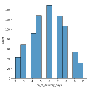
29     6
535    3
695    8
557    5
836    9
Name: no_of_delivery_days, dtype: int64

Copy to Clipboard

array([[ 1.26234643,  0.9764221 ,  0.22314994,  0.44560793, -1.83483918,
        -1.20757264],
       [ 0.12700257, -0.14113953,  0.96411821,  0.52720777,  1.18937949,
         1.43120235],
       [-0.06301307, -0.53241671, -0.97728689, -0.26314488, -1.79967385,
        -1.1972752 ],
       ...,
       [ 1.23018703,  1.18247717,  0.81514727,  1.37584601, -0.18206851,
         0.78864196],
       [-1.14424485, -1.45886269,  0.96411821,  0.52720777,  1.18937949,
         1.43120235],
       [-0.97055635, -0.566122  , -0.15123758, -0.48696156, -0.42822585,
        -0.54473421]])

Copy to Clipboard

array([[ 1.26234643,  0.9764221 ,  0.22314994,  0.44560793, -1.83483918,
        -1.20757264],
       [ 0.12700257, -0.14113953,  0.96411821,  0.52720777,  1.18937949,
         1.43120235],
       [-0.06301307, -0.53241671, -0.97728689, -0.26314488, -1.79967385,
        -1.1972752 ],
       ...,
       [ 1.23018703,  1.18247717,  0.81514727,  1.37584601, -0.18206851,
         0.78864196],
       [-1.14424485, -1.45886269,  0.96411821,  0.52720777,  1.18937949,
         1.43120235],
       [-0.97055635, -0.566122  , -0.15123758, -0.48696156, -0.42822585,
        -0.54473421]])

Copy to Clipboard

Decision Tree Regression Delivery Days Prediction Y hat: [6. 3. 8. 5. 9. 6. 6. 7. 8. 5.]
Decision Tree Regression Delivery Days Actual Y:  [6, 3, 8, 5, 9, 6, 6, 7, 8, 5]

Copy to Clipboard

Decision Tree Regression Delivery Days Mean Squared Error:  0.0
Decision Tree Regression Delivery Days Root Mean Squared Error:  0.0

Copy to Clipboard

array([2.74772633, 2.88530761, 2.97489496, 2.92831009, 3.01662063,
       3.0228298 , 2.88097206, 3.01869177, 3.3015148 , 2.63865496])

Copy to Clipboard

Scores:  [2.74772633 2.88530761 2.97489496 2.92831009 3.01662063 3.0228298
 2.88097206 3.01869177 3.3015148  2.63865496]
Mean:  2.941552300893142
Standard deviation:  0.16887883559008862

Conclusion on Scikit Learn – Decision Tree Regression Model:

Decision Tree Regression is a powerful model and it works great in complex nonlinear relationships in the data.
Decision Tree Regression model is not performing well on delivery days prediction, however you may conclude that it is a good predicting model because of accurate prediction, mean squared error and root mean squared error also shows zero.
The model is overfitting the data very badly.
Scores shows in the range of 2.6 to 3.3.
We will check in Random Forest Regression with same data as it was doing a pretty good job on Customer Price Prediction and it was giving accurate results and less errors.